SPY 단타 전략 백테스트 : rsi powerzones

강환국님 유튜브 동영상에서 rsi powerzones라는 단타전략을 알게되었다. 매우 간단한 전략이라서 backtrader 공부도할겸 백테스트해보았다.

1) 거래로직

거래로직은 다음의 매수, 매도신호에 따라 매매한다.

• 매수 신호
  • 현재가격이 200일 이동평균선보다 위에 있고
  • RSI(4)가 30미만으로 떨어지면 Buy
  • RSI(4)가 25미만으로 떨어지면 추가 매수
    • (추가매수하는 부분은 약간 복잡해서 코드상으로는 스킵하고 실험)
• 매도 신호
  • RSI(4)가 55이상이면 Sell

2) 실험결과

전체기간 : 1993년 ~ 2021년 7월 31일

먼저 SPY데이터를 구할 수 있는 전체 구간에 대한 테스트 결과이다. 위에서 두번째 박스에 파란색은 이긴 거래, 빨간색은 진 거래(손실을 본 거래)를 의미한다.

1993년 11월 12일 ~ 2021년 7/31

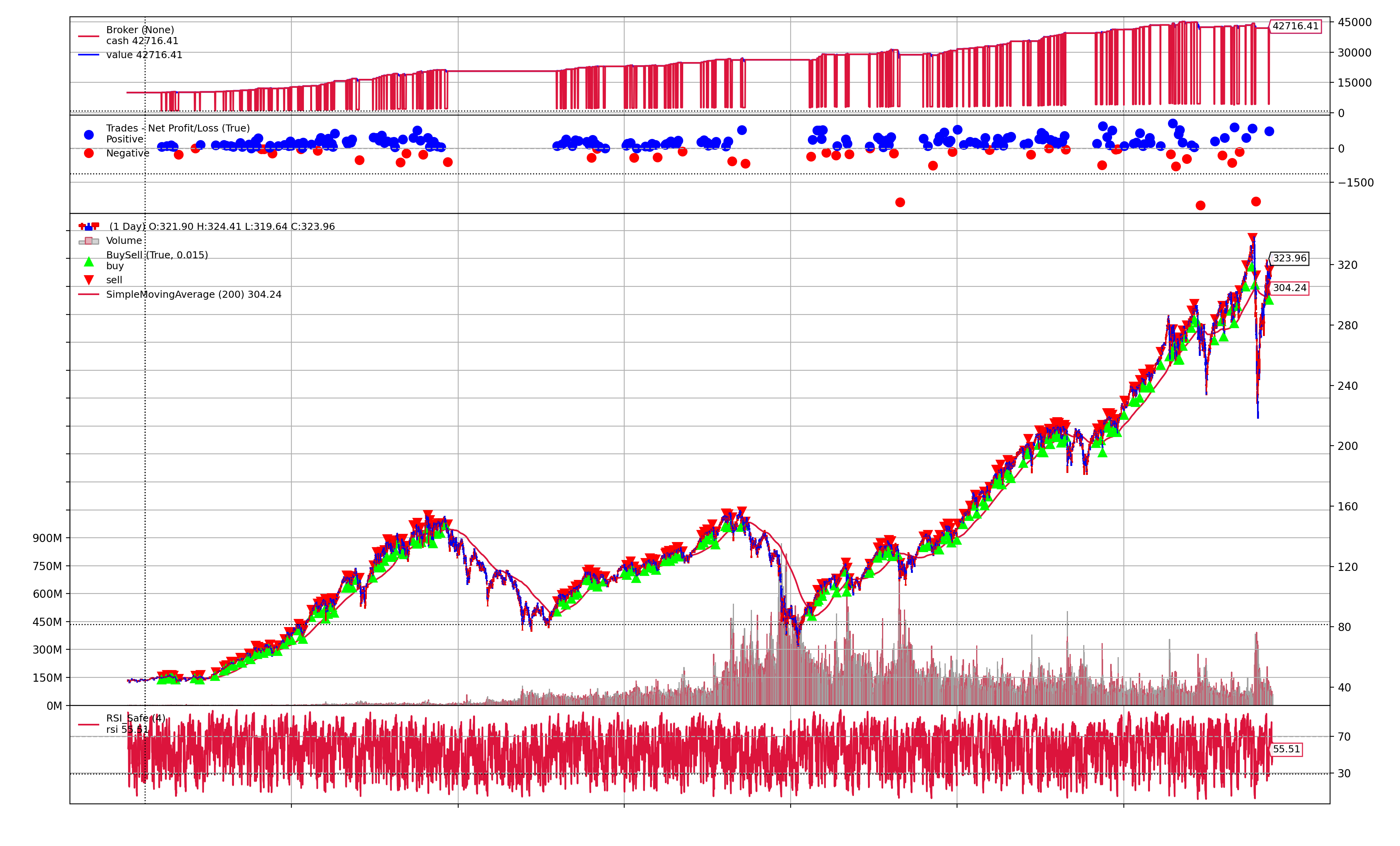
• 딱 봐도 파란색이 빨간색보다 훨씬 많다. 승률이 높은 전략임을 알 수 있다.
• 그러나 빨간색이 밑으로 내려살때가 많다. 손익비로 보면 좋은 전략이 아닌것같다.
• 수치로 연산해본 승률과 손익비는 다음과같다.
  • 승률 : 81%, 손익비 : -0.71
  • 이기는 거래가 많지만 이길때 조금먹고, 깨질때 많이깨진다는 뜻이다.

상승장 : 1993년 ~ 1999년 12월 31일

이번에는 대세상승장인 1990년대에 대해서만 돌려봤다.

1993년 ~ 1999년

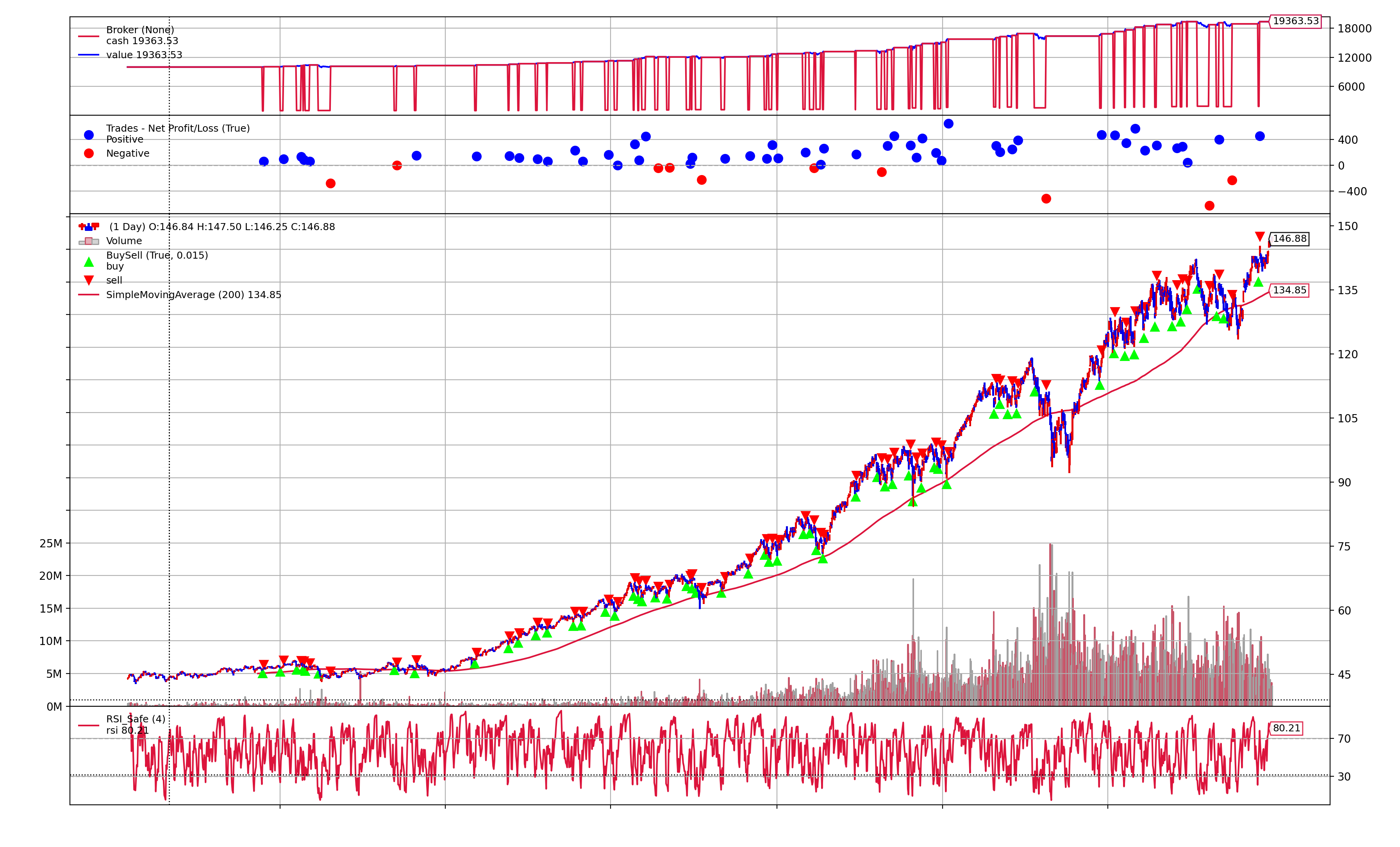
• 이 구간에서도 승률은 높고 손익비는 낮다. 
• 승률 84%, 손익비 -1.04

횡보장 : 2000년 1월 1일 ~ 2010년 12월 31일

미국주식이 죽을 쑤던 2000년대로 구간을 짤라서 테스트해봤다. (이 결과는 좀 괜찮다!)

 

2000년대 SPY

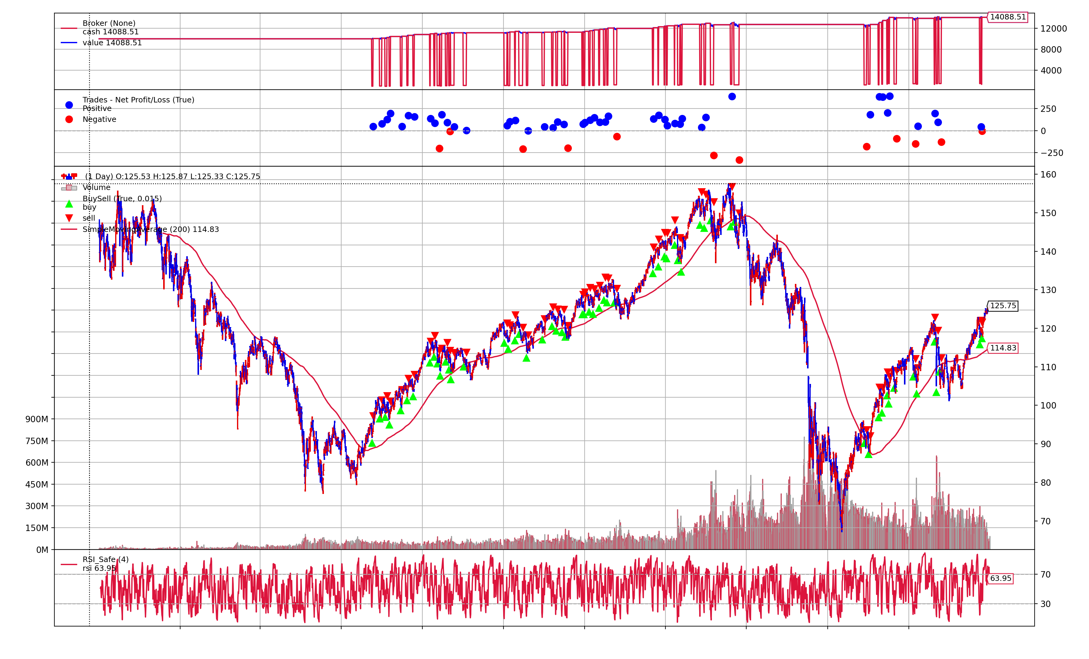
• 전체 구간으로 보면 횡보장이지만 중간의 상승장에서만 거래하도록 로직이 설계되어있다.
• 승률이 높고 손익비가 낮은것은 이전의 결과와 동일하다.
  • 승률 : 78%, 손익비 : -0.91
  • 횡보장에서 이 정도면 괜찮은 듯..?

 

정리

테스트 구간	승률	손익비
1993년 ~ 1999년 (상승장)	84%	-1.04
2000년 ~ 2010년 (횡보장)	78%	-0.91
2011년 ~ 2021년 7월 (상승장)	79%	-0.75
전체 구간 (1993년 ~ 2021년 7월)	81%	-0.71

테스트 구간을 나누어봐도 승률이 유지된다는 것 이 전략의 장점인 것 같다. 그러나 손익비가 낮고, 거래가 잦다는 (그래서 단타 전략임...) 점이 단점이다.

 

 

python 소스코드

	import FinanceDataReader as fdr
	import backtrader as bt
	# Create a Stratey
	class TestStrategy(bt.Strategy):
	params = (
	('maperiod', 200),
	('rsi_period', 4),
	('rsi_entry', 30),
	('rsi_exit', 55),
	)
	def __init__(self):
	# Keep a reference to the "close" line in the data[0] dataseries
	self.dataclose = self.datas[0].close
	# To keep track of pending orders and buy price/commission
	self.order = None
	# Add a MovingAverageSimple indicator
	self.sma = bt.indicators.SimpleMovingAverage(self.datas[0], period=self.params.maperiod)
	self.rsi = bt.indicators.RSI_Safe(self.datas[0], period=self.params.rsi_period)
	self.n_wins = 0
	self.n_losses = 0
	self.profits = 0
	self.losses = 0
	# 승률, 평균 이익계산?
	def notify_trade(self, trade):
	if not trade.isclosed:
	return
	self.log('OPERATION PROFIT, GROSS %.2f, NET %.2f' %
	(trade.pnl, trade.pnlcomm))
	if trade.pnl > 0:
	self.n_wins += 1
	self.profits += trade.pnl
	else:
	self.n_losses += 1
	self.losses += trade.pnl
	def next(self):
	# Simply log the closing price of the series from the reference
	self.log('Close, %.2f' % self.dataclose[0])
	# Check if an order is pending ... if yes, we cannot send a 2nd one
	if self.order:
	return
	# Check if we are in the market
	if not self.position:
	# Not yet ... we MIGHT BUY if ...
	if self.dataclose[0] > self.sma[0] and self.rsi[0] <= self.p.rsi_entry:
	# 2003-05-19, BUY CREATE, 92.65
	# BUY, BUY, BUY!!! (with all possible default parameters)
	self.log('BUY CREATE, %.2f' % self.dataclose[0])
	# Keep track of the created order to avoid a 2nd order
	self.order = self.buy()
	else:
	if self.rsi[0] >= self.p.rsi_exit:
	# SELL, SELL, SELL!!! (with all possible default parameters)
	self.log('SELL CREATE, %.2f' % self.dataclose[0])
	# Keep track of the created order to avoid a 2nd order
	self.order = self.sell()
	def stop(self):
	win_ratio = self.n_wins / (self.n_wins + self.n_losses)
	avg_profit = self.profits / self.n_wins
	avg_loss = self.losses / self.n_losses
	profit_loss_ratio = avg_profit / avg_loss
	expected_profit_per_trade = win_ratio * avg_profit + (1-win_ratio) * avg_loss
	print(f"win_ratio: {win_ratio:.2f}, "
	f"profit_loss_ratio: {profit_loss_ratio:.2f}, "
	f"expected_profit_per_trade: {expected_profit_per_trade:.2f}")
	if __name__ == '__main__':
	cerebro = bt.Cerebro()
	cerebro.addstrategy(TestStrategy)
	# spy = fdr.DataReader('SPY', '2000-01-01', '2005-05-30')
	spy = fdr.DataReader('SPY', '2000-01-01', '2010-12-31')
	# spy = fdr.DataReader('SPY', '1990-01-01', "1999-12-31")
	data = bt.feeds.PandasData(dataname=spy)
	cerebro.adddata(data)
	# Set our desired cash start
	cerebro.broker.setcash(10000.0)
	# Add a FixedSize sizer according to the stake
	cerebro.addsizer(bt.sizers.PercentSizer, percents=90)
	# Print out the starting conditions
	print('Starting Portfolio Value: %.2f' % cerebro.broker.getvalue())
	# Run over everything
	cerebro.run()
	# Print out the final result
	print('Final Portfolio Value: %.2f' % cerebro.broker.getvalue())
	cerebro.plot(style='candlestick', barup="red", bardown="blue")
	# 1993-11-12 ~ 2021-07-30
	# win_ratio: 0.81, profit_loss_ratio: -0.71, expected_profit_per_trade: 166.32
	# 1993-11-12 ~ 1999-12-31
	# win_ratio: 0.84, profit_loss_ratio: -1.04, expected_profit_per_trade: 151.02
	# 2000-01-01 ~ 2010-12-31
	# win_ratio: 0.78, profit_loss_ratio: -0.91, expected_profit_per_trade: 69.30
	# 2011-01-01 ~ 2021-07-30
	# win_ratio: 0.79, profit_loss_ratio: -0.75, expected_profit_per_trade: 75.95

view raw spy_rsi_power_zones hosted with ❤ by GitHub

 

참고자료

• 강환국님 유튜브 동영상